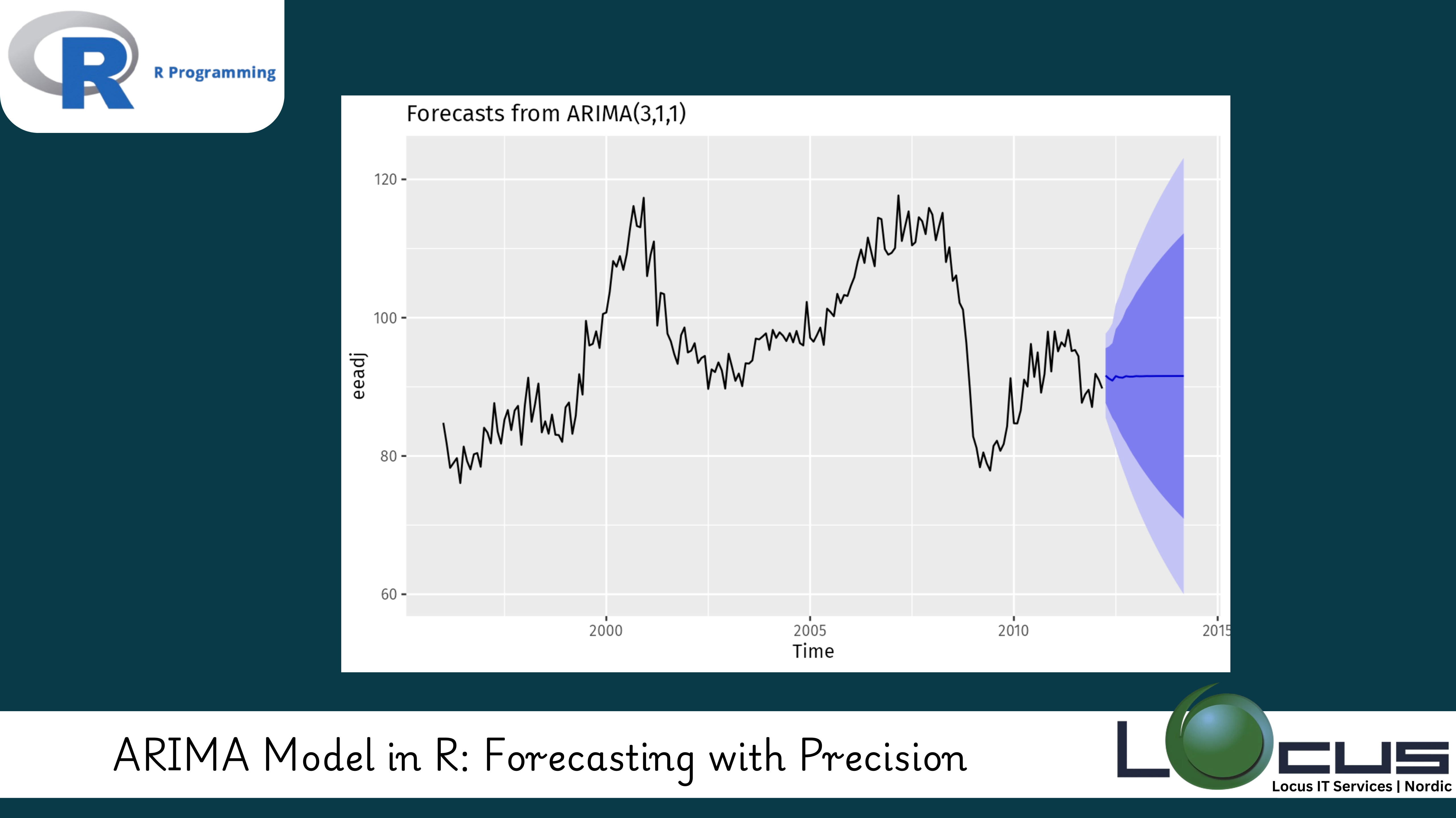
For Every Business, Time series forecasting is essential for many industries—whether predicting sales, stock prices, weather patterns, or customer demand. One of the most powerful and widely used techniques for time series forecasting is ARIMA (AutoRegressive Integrated Moving Average). In this blog post, we will explore ARIMA Model in R, a robust method that combines autoregressive (AR) and moving average (MA) components with differencing to model time series data effectively.
What is ARIMA?
ARIMA Model in R is a popular statistical model used for analyzing and forecasting time series data. It is a combination of three key components: (Ref: Scaling ML Pipelines in R: Best Practices & Strategies)
- Autoregressive (AR): The ARIMA Model in R uses the relationship between an observation and a specified number of lagged observations (previous values in the series).
- Integrated (I): This component involves differencing the series to make it stationary. Stationarity is crucial for ARIMA models, as they assume the statistical properties of the series (mean, variance, and autocovariance) do not change over time.
- Moving Average (MA): This component models the relationship between an observation and a residual error from a moving average model applied to lagged observations.
ARIMA Model in R is often referred to by its parameters (p, d, q):
- p: The number of lag observations in the autoregressive model (AR).
- d: The number of times the series is differenced to make it stationary (I).
- q: The number of lagged forecast errors in the moving average model (MA).
Why Use ARIMA in Time Series Forecasting?
ARIMA is an excellent tool for forecasting time series data when:
- The data shows trends or patterns that need to be accounted for.
- The time series is univariate (consists of a single variable).
- The data can be made stationary (the mean and variance do not change over time).
Its advantages include:
- Flexibility: ARIMA can model a wide range of time series data.
- Simplicity: With just three parameters (p, d, q), ARIMA is relatively simple to understand and implement.
- Performance: When properly tuned, ARIMA can produce highly accurate forecasts.
How to Implement ARIMA Model in R
R provides several tools for implementing ARIMA, most notably through the forecast package. Below are the basic steps to apply ARIMA Model in R to your time series data in R.
1. Install and Load Required Packages
To begin, install and load the forecast package, which contains the auto.arima() function for automatically fitting ARIMA models.

2. Load Your Data
Next, you need to load your time series data into R. ARIMA Model in R supports many formats, including CSV files, and it provides a ts() function for creating time series objects.

3. Check for Stationarity
Before applying ARIMA, the data must be stationary. You can visually inspect the data and use statistical tests like the Augmented Dickey-Fuller (ADF) test to check for stationarity.

If the series is not stationary, you can difference it using the diff() function.

4. Fit the ARIMA Model
R’s auto.arima() function automatically selects the optimal p, d, and q values based on AIC (Akaike Information Criterion) or BIC (Bayesian Information Criterion). It fits the ARIMA model and returns the best parameters.

5. Model Diagnostics
After fitting the model, it’s essential to check the residuals (errors) for randomness. If the residuals show patterns, the model may need refinement.

6. Forecasting
Once the model is built and validated, you can use it to make forecasts. The forecast() function allows you to predict future values and visualize the results.

Practical Use Cases for ARIMA in R
ARIMA is widely used in various fields, and here are a few examples:
1. Sales Forecasting
Retailers often use ARIMA to predict sales trends and optimize inventory management. By fitting ARIMA to historical sales data, businesses can forecast future demand with high accuracy, helping them prepare for seasonal variations and avoid overstocking or stockouts.
2. Stock Price Prediction
ARIMA can be applied to historical stock prices to predict future prices. Although stock prices are influenced by many factors, ARIMA can capture trends and patterns that help investors make informed decisions.
3. Energy Consumption Forecasting
Utility companies can use ARIMA to predict future energy demand based on historical usage data. This enables better planning and resource allocation, ensuring that energy supply meets demand.
4. Economic Indicators
Government agencies and financial institutions often use ARIMA for forecasting economic indicators such as inflation rates, GDP growth, or unemployment rates. Accurate predictions help policymakers make informed decisions.
Challenges and Limitations of ARIMA
While ARIMA is a powerful tool, it does have limitations:
- Stationarity: ARIMA Model in R assumes that the time series is stationary. If the series has complex patterns or structural breaks, other models may be more appropriate.
- Linear Assumptions: ARIMA Model in R assumes linear relationships, which may not always be the case in real-world data.
- Long-Term Forecasting: ARIMA Model in R is better suited for short-term forecasting. For long-term forecasts, it may not always capture complex patterns accurately.
Final Thoughts
ARIMA Model in R is a robust and efficient method for time series forecasting. It is highly effective for predicting future values based on historical data and capturing trends, seasonality, and autocorrelation. By following best practices such as ensuring stationarity, validating your model, and performing diagnostics, you can harness the full power of ARIMA Model in R to make data-driven predictions across a wide range of applications.
Whether you’re forecasting sales, predicting stock prices, or estimating demand for resources, ARIMA Model in R offers the tools necessary for accurate and actionable insights. (Ref: Locus IT Services)


