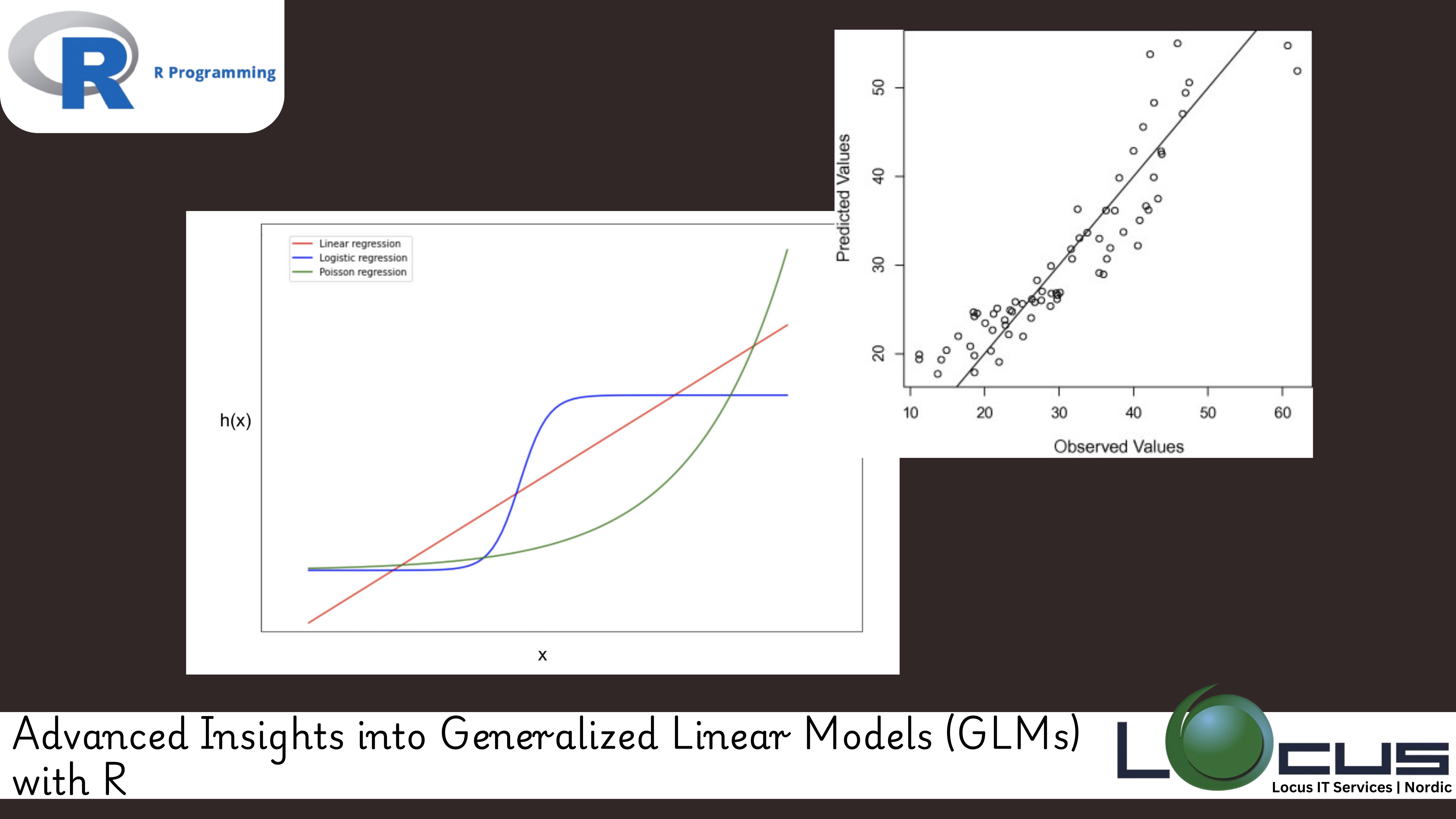
For Every Business, Statistical modeling is a cornerstone of data science, and one of the most versatile tools in a statistician’s arsenal is the Generalized Linear Model (GLM). GLMs extend linear models to allow for response variables that are not normally distributed, making them particularly useful for analyzing data in a variety of domains, including biology, finance, healthcare, and more. In R, GLMs are implemented via the powerful glm() function, which provides flexibility and ease of use.
This blog will introduce the concept of GLMs, their components, common applications, and how to implement them in R.
What Are Generalized Linear Models?
A Generalized Linear Model (GLM) is a flexible extension of the traditional linear regression model. While linear regression assumes a continuous response variable that follows a normal distribution, GLMs generalize this framework by accommodating different types of response variables, such as binary, count, or categorical outcomes. (Ref: Using ggplot2 for Model Diagnostics in R)
A GLM consists of three main components:
- Random Component: The distribution of the response variable (e.g., normal, binomial, Poisson).
- Systematic Component: The linear predictor, which is a linear combination of the explanatory variables.
- Link Function: A function that relates the expected value of the response variable to the linear predictor.
Why Use GLMs?
GLMs are particularly useful when:
- The response variable does not follow a normal distribution (e.g., binary or count data).
- The relationship between the response and predictors is non-linear.
- You want to model probabilities, counts, or other specialized outcomes.
Common applications of GLMs include:
- Logistic regression for binary outcomes.
- Poisson regression for count data.
- Multinomial regression for categorical outcomes.
Types of GLMs
- Logistic Regression: Used when the response variable is binary (e.g., 0 or 1, success or failure).
- Example: Predicting whether a patient has a disease (yes/no).
- Poisson Regression: Used for count data where the response variable represents the number of occurrences of an event.
- Example: Modeling the number of customer complaints received per day.
- Gamma Regression: Used for modeling positive continuous data with a skewed distribution.
- Example: Modeling time to failure for a machine.
- Multinomial Regression: An extension of logistic regression for categorical response variables with more than two levels.
- Example: Predicting the preferred choice of a product from multiple options.
Components of a GLM
- Response Variable: The variable you’re trying to predict. It could be binary, count-based, or categorical.
- Predictor Variables: Independent variables or features used to predict the response variable.
- Link Function: Transforms the expected value of the response variable into a linear form. Examples include:
- Logit link for logistic regression.
- Log link for Poisson regression.
- Identity link for linear regression.
Implementing GLMs in R
R provides the glm() function to fit Generalized Linear Models. Here’s a step-by-step guide to using GLMs in R:
1. Logistic Regression
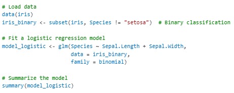
Logistic regression is used for binary outcomes. For example, predicting whether a patient has diabetes based on their health metrics.

The family = binomial argument specifies logistic regression.
2. Poisson Regression
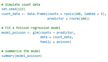
Poisson regression is used for count data. For example, modeling the number of customer complaints received per day.

The family = poisson argument specifies Poisson regression.
3. Gamma Regression
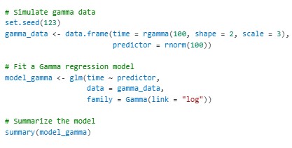
Gamma regression is used for modeling positive continuous data. For example, modeling the time to failure for a machine.

The family = Gamma(link = "log") argument specifies Gamma regression with a log link.
Interpreting GLM Output
Key components of a GLM summary in R include:
- Coefficients: The estimated effect of each predictor variable.
- Standard Error: The uncertainty associated with each coefficient estimate.
- z-value and p-value: Indicate the significance of the predictors.
- Deviance and AIC: Metrics for model fit and comparison.
For logistic regression, coefficients are often interpreted in terms of odds ratios using the exponential function (exp()).
Challenges in Using GLMs
- Selecting the Right Link Function: Choosing an inappropriate link function can lead to poor model performance.
- Overdispersion: In Poisson regression, variance greater than the mean (overdispersion) can affect the results.
- Multicollinearity: Highly correlated predictors can distort coefficient estimates.
Best Practices for GLMs
- Data Preparation: Ensure the response variable matches the chosen family (e.g., binary for logistic regression).
- Model Validation: Use techniques like cross-validation to evaluate model performance.
- Diagnostics: Check residuals, leverage, and goodness-of-fit metrics to validate the model.
- Transform Predictors: If necessary, apply transformations to improve model fit.
Final Thoughts
Generalized Linear Models (GLMs) are a powerful framework for handling diverse data types and distributions, making them indispensable in modern data science. With R’s glm() function, you can easily implement logistic regression, Poisson regression, and other GLMs to solve real-world problems across domains.
By understanding the components of Generalized Linear Model, selecting the right link function, and validating your models, you can harness the full potential of GLMs for robust and reliable statistical analysis. Whether you’re analyzing binary outcomes, count data, or more complex relationships, GLMs in R are a go-to tool for statistical modeling. (Ref: Locus IT Services)


